• Preface
• Dynamic Programming

• Policy Iteration

  • Steps
  • Algorithm
• Policy Evaluation - Prediction * Points to consider
• Policy Improvement - Control
• Value Iteration * Points to consider * Pseudo Code
• Generalised Policy Iteration (GPI)
• References

Preface

There are two basic steps for solving any RL problem.

• Policy evaluation refers to the iterative computation of the value functions for a given policy.
• Policy improvement refers to finding an improved policy given the value function for an existing policy.

Two basic approaches to solve an RL problem:

• Policy Iteration and
• Value Iteration

Both these techniques use these two steps repeatedly to arrive at optimality. Either of these can be used to reliably compute optimal policies and value functions given complete knowledge of the MDP.

The basic assumption of model based methods is that the model $p(s', r|s, a)$ is available.

Dynamic Programming

Dynamic Programming (DP) is a method of solving complex problems by breaking them into sub-problems. It solves the sub-problems and stores the solution of sub-problems, so when next time same subproblem arises, one can simply look up the previously computed solution.

Why should you apply dynamic programming to solve Markov Decision Process?

1. Bellman equations are recursive in nature. You can break down Bellman equation to two parts – (i) optimal behaviour at next step (ii) optimal behaviour after one step
2. You can cache the state value and action value functions for further decisions or calculations.

Policy Iteration

Steps

1. Initialize a policy randomly

2. Policy Evaluation:

   1. Measure how good that policy is by calculating the state-values $v_{\pi}(s)$ corresponding to all the states until the state-values are converged.
   2. Also known as the prediction problem.

3. Policy Improvement:

   1. Make changes in the policy you evaluated in the policy evaluation step.
   2. Also known as the control problem.

Algorithm

In the policy iteration algorithm, you first initialise a policy $\pi$ randomly. Next, you evaluate the policy according to the Bellman equation. For each state s, you compute:

$v_{\pi}(s) = \sum_{a}\pi(a|s)[\sum_{s'}\sum_{r}p(s',r|s,a)(r + \gamma v_{\pi}(s'))]$

The meaning of the three summations:

• Summation over all possible actions which the agent can take when in state s following policy $\pi$.
• Once the initial state and action are fixed, the summation of probabilities of all possible next states and rewards.

$v_{\pi}(s)$ is evaluated until the state-values are converged for the policy $\pi$; after that you improve the policy.

How do you improve the state-value function?

You do this by following a greedy approach, i.e, by taking the best action at every state. The action with the maximum state-action value $q_{\pi}(s, a)$ is the best action. The improved policy $\pi'$ is:

$\pi'(a|s) = \begin{cases} 1 & a = \text{argmax}_a[\sum_{s'}\sum_{r}p(s',r|s,a)(r + \gamma v_{\pi}(s'')] \\ 0 & \text{otherwise} \end{cases}$

To calculate the $v_{\pi}(s)$ in the policy evaluation step, you need the value of $v_{\pi}(s')$. But you don't have any estimate for $v_{\pi}(s')$. Thus, apart from initializing the policy, you also initialize the state-value function randomly.

Let's say that you have N states. In the policy evaluation step, you can write the value function for each state as:

${v_{\pi}(s_1) = \sum_{a}\pi(a|s_1)\sum_{s'}\sum_{r}p(s',r|s,a)(r + \gamma v_{\pi}(s'))}$

${v_{\pi}(s_2) = \sum_{a}\pi(a|s_2)\sum_{s'}\sum_{r}p(s',r|s,a)(r + \gamma v_{\pi}(s'))}$

${v_{\pi}(s_3) = \sum_{a}\pi(a|s_3)\sum_{s'}\sum_{r}p(s',r|s,a)(r + \gamma v_{\pi}(s'))}$

. . .

${v_{\pi}(s_N) = \sum_{a}\pi(a|s_N)\sum_{s'}\sum_{r}p(s',r|s,a)(r + \gamma v_{\pi}(s'))}$

There are N variables - $v_{\pi}(s_1), v_{\pi}(s_2), ..., v_{\pi}(s_N)$. This is a system of simultaneous linear equations in N variables. Theoretically, you can solve it to get the state-value functions. However, practically the number of states is generally quite large and so we user alternate iterative techniques to solve this.

The stopping condition for Policy Iteration is:

• For each state $v_{\pi}(s) = v_{\pi'}(s)$
• The value of a state for the improved policy should be the same for the policy we started with.

Policy Evaluation - Prediction

Let's rearrange the equations. The equation:

$v_{\pi}(s) = \sum_{a}\pi(a|s)[\sum_{s'}\sum_{r}p(s',r|s,a)(r + \gamma v_{\pi}(s'))]$

can be rewritten as

$v_{\pi}(s_1) = c_1\times v_{\pi}(s_1)+c_2\times v_{\pi}(s_2)+c_3\times v_{\pi}(s_3) + ...$

Hence the system of linear equations can be written as:

$v_{\pi}(s_1) = c_1\times v_{\pi}(s_1)+c_2\times v_{\pi}(s_2)+c_3\times v_{\pi}(s_3) + ...$

$v_{\pi}(s_2) = d_1\times v_{\pi}(s_1)+d_2\times v_{\pi}(s_2)+d_3\times v_{\pi}(s_3) + ...$

$v_{\pi}(s_3) = e_1\times v_{\pi}(s_1)+e_2\times v_{\pi}(s_2)+e_3\times v_{\pi}(s_3) + ...$

This can be further simplified as:

A constant matrix*$[v_{\pi}(s_1), v_{\pi}(s_2),...]$ = another constant matrix. So, the policy evaluation equation could be written as:

$A\vec v = c$

Where $\bold A$ is a function of policy, the model of the environment and discount factor and c is a function of policy, model of the environment and reward.

These equations could be solved using matrix inverse. This approach is computationally expensive and is not suitable when the number of states is huge.

The other method is to iteratively solve for $v_{\pi}(s)$. You \start with initialised values for $v_{\pi}(s)$ and then compute the new values using the policy evaluation equation. And then you use the new values to re-compute the values $v_{\pi}(s)$. You continue to do this until $v_{\pi}(s)$ shows convergence, i.e., value get stabilised for a particular policy.

Points to consider

• We don't need to initialize $v_{\pi}(s)$ for closed form solution. We can just solve the equations.
• Policy evaluation equation is written for each state. While solving for value functions, the number of actions won't affect the number of equations. If there are 50 states in RL problem and 4 actions for each state, then number of equations will be 50.
• We use iterative methods for large state spaces (all practical problems have large state spaces) as closed form (inverse matrix) calculation is too expensive.

Policy Improvement - Control

Once the value function $v_{\pi}(s)$ is evaluated, the agent improves the policy. The improvement is made greedily with respect to the current value function. In state s, that action is chosen which has the maximum state-action value, i.e. maximum $q_{\pi}(s, a)$ value:

$\pi'(a|s) = \begin{cases} 1 & a = \text{argmax}_a[\sum_{s'}\sum_{r}p(s',r|s,a)(r + \gamma v_{\pi}(s'')] \\ 0 & \text{otherwise} \end{cases}$

If there is no improvement in the policy, then the agent is already at the optimal policy. Else, we need to evaluate the improved policy until the state-values converge and then perform the policy improvement step on top of it. These steps are repeated until there is no further improvement in the policy.

Value Iteration

You can compute the maximum value of a state by comparing the different actions possible in that state - the action which results in the max state-value is the optimal action. This is the major idea behind Value Iteration algorithm.

In value iteration, instead of running the policy evaluation step till the state-values converge, you perform exactly one update, calculating the state-values. These state-values are corresponding to the action that yields the maximum state-action value. The state-value function is a greedy choice among all the current actions:

$v(s) = \max_{a}[\sum_{s'}\sum_{r}p(s',r|s,a)(r + \gamma v(s'))]$

Policy improvement is an implicit step in state-value function update. The update step combines the policy improvement and (truncated) policy evaluation steps.

Points to consider

• Value Iteration is computationally less expensive when compared with policy iteration as the entire sweep till state-value function stabilisation need not be done
• The optimal value function obtained from Policy and Value Iteration will be the same. They both will converge to give the same results
• The update is greedy in terms of best action to be taken from state s

Pseudo Code

(a) Initialise value functions for each state, i.e., v(s) for all s.

(b) Repeat:

• Select a state, s
• Calculate the value for each action starting from state s, i.e., q(s, a)
• Select the highest value among the q-values calculated in the previous step.
• Store v(s)

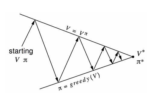
Generalised Policy Iteration (GPI)

Policy Iteration and Value Iteration are two sides of a coin.

In policy iteration, you complete the entire policy evaluation to get the estimates of value functions for a given a policy and then use those estimates to improve the policy. And then repeat these two steps, until you arrive at optimal state value function.

In value iteration, for every state update, you’re doing a policy improvement, i.e., updating the state value by picking the most greedy action using current estimates of state-values.

Generalised Policy Iteration (GPI) is a class of algorithms that pans out the entire range of strategies that fall between Policy Iteration & Value Iteration. A GPI is basically the following two steps running in a loop

1. Updates based on current values
2. Policy improvement

A GPI becomes:

• Policy Iteration: When Policy Evaluation is done till convergence and then one step of Policy Improvement.
• Value Iteration: When one step of Policy Evaluation is done and then one step of Policy Improvement.

References

• Dynamic Programming - Stanford