• Purpose

• Exponential Functions

  • Laws of Exponents

• Logarithm Property

  • Note
  • Solving Equations containing exponents

  • Properties of Logarithms

    • Product Property
    • Quotient Property
    • Power Property
    • More Rules
• Linear Regression vs Logistic Regression
• Examples of Logistic Regression
• Binary classification

• Sigmoid function

  • Formula
  • Best fit Sigmoid Curve
• Building a logistic regression model in Python
• Odds and Log Odds
• Summary

• Multivariate Logistic Regression

  • Why checking Churn Rate is Important
  • Why we only use transform on test set
• Model Building

• Confusion Matrix and Accuracy

  • Accuracy
  • Creating confusion matrix

• Interpreting the Model

  • Questions
• Summary - Multivariate Logistic Regression

• Metrics

  • Confusion Matrix
  • Accuracy
  • Sensitivity
  • Specificity
  • False Positive Rate
  • Negative Predictive Value
  • Positive Predictive Value
  • Receiver Operating Characteristic Curve - ROC Curve
  • Questions
  • Precision
  • Recall
  • Questions
• Summary - Steps of Building a Classification Model
• Takeaways

• Measures of Discriminative Power

  • Gain Chart
  • Lift
  • KS Statistic
• References

Purpose

My notes on Logistic Regression

Exponential Functions

Laws of Exponents

• $x^a.x^b = x^{a+b}$
• $(xy)^a=x^a.y^a$
• $\frac{x^a}{x^b}=x^{a−b}; x \neq 0$
• $(\frac{x}{y})^a=\frac{x^a}{y^a}; y \neq 0$
• $x^0 = 1; x \neq 0$
• $\frac{1}{x^a}=x^{-a}; x \neq 0$
• $(x^a)^b = x^{a*b}$

---

Logarithm Property

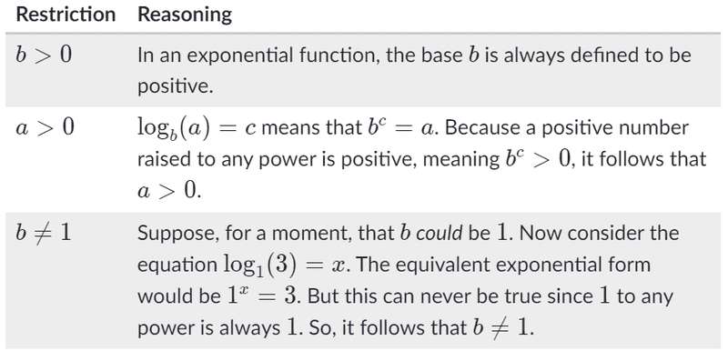
Logarithm helps us redefine exponents. $\log_{b}a$ means what power does b have to be raised to, to get a.

$log_{b}(a) = c \Leftrightarrow b^c = a;$ where

• b is base
• c is exponent
• a is argument

Note

When rewriting an exponential equation in log form or a log equation in exponential form, it is helpful to remember that the base of the logarithm is the same as the base of the exponent.

Read more about logarithms here and here

Solving Equations containing exponents

Q: $6^x = 20$

• $6 = 10^{log6}$
• $20 = 10^{log20}$
• $(10^{log6})^x = 10^{log20}$
• $10^{log6.x} = 10^{log20}$
• $x.\log6 = \log20$
• $x=\frac{log20}{log6} \approx 1.67$

Properties of Logarithms

Product Property

$\log_{b}ac = \log_{b}a + log_{b}c;$ where a,b,c are positive numbers, $b \neq 1$

Quotient Property

$\log_{b}\frac{a}{c} = \log_{b}a - log_{b}c;$ where a,b,c are positive numbers, $b \neq 1$

Power Property

$\log_{b}a^c = c.\log_{b}a$ where c is a real number, a and b are positive numbers, $b \neq 1$

More Rules

$\log_{b}c = \frac{log_{z}c}{log_{z}b}$

---

Linear Regression vs Logistic Regression

Linear Regression	Logistic Regression
numeric output	categorical output

Examples of Logistic Regression

1. Finance Company want sto know whether a customer will default or not
2. Predicting an email is spam or not
3. Categorizing email into promotional, personal and official

Binary classification

1. Two possible outputs

2. Examples:

   • customer will default or not
   • email spam or not
   • a user is a robot or not

Sigmoid function

sigmoid curve has all the properties you would want in a binary classification problem and hence it's good for such models.

• extremely low values in the start
• extremely high values in the end
• intermediate values in the middle

Formula

$y = prob(x) = \frac{1}{1+e^{(-\beta_{0} + \beta_{1}x)}}$

Best fit Sigmoid Curve

Likelihood function Product of $(1-P_{ineg})(P_{ipos})$ for i = 1 to N, is called the Likelihood function

Building a logistic regression model in Python

We can use statsmodel to build a logistic regression model

import statsmodel.api as sm logm1 = sm.GLM(y,(sm.add_constant(X)), family = sm.families.Binomial()) logm1.fit().summary()

The coef column gives us the value of $\beta_{0}$ and $\beta_{1}$

Odds and Log Odds

This equation: $P = \frac{1}{1+e^{(-\beta_{0} + \beta_{1}x)}}$ is difficult to interpret.
We can simplify it by using Odds which is given as:

$\frac{P}{1-P} = e^{\beta_{0} + \beta_{1}x}$

We interpret odds as:

$\newline P(EventHappens) = Odds*P(EventDoesNotHappen)\newline or\;P = Odds*(1-P)$

Moreover, with every linear increase in X, the increase in odds is multiplicative

The Log Odds can then be obtained by applying $\ln$ (i.e. natural log or log with base e or $\log_{e}$)

$\ln{\frac{P}{1-P}} = \beta_{0} + \beta_{1}x$

As we can see the RHS is the equation of a straight line, hence Log Odds follows a linear relationship w.r.t X.

Summary

• Simple boundary decision approach is not good for classification problems
• Sigmoid function gives us a good approximation of the probability of one of the classes being selected based on the input
• The process where you vary the betas until you find the best fit curve for the probability of an event occurring, is called logistic regression.
• The equation for likelihood is complex, and hard to interpret, hence we use Odds $(\frac{1}{1-P})$ and Log Odds $(\ln\frac{1}{1-P})$
• The Log Odds vs X graph is linear in nature as it follows the equation of a straight line

---

Multivariate Logistic Regression

$P = \frac{1}{1-e^{-(\beta_{0} + \beta_{1}x_{1} + ... + \beta_{1}x_{n})}}$

Why checking Churn Rate is Important

The reason for having a balance is simple. Let’s do a simple thought experiment - if you had a data with, say, 95% not-churn (0) and just 5% churn (1), then even if you predict everything as 0, you would still get a model which is 95% accurate (though it is, of course, a bad model). This problem is called class-imbalance and you'll learn to solve such cases later.

Why we only use transform on test set

The 'fit_transform' command first fits the data to have a mean of 0 and a standard deviation of 1, i.e. it scales all the variables using:

$X_{scaled} = \frac{X − \mu}{\sigma}$

Now, once this is done, all the variables are transformed using this formula. Now, when you go ahead to the test set, you want the variables to not learn anything new. You want to use the old centralisation that you had when you used fit on the train dataset. And this is why you don't apply 'fit' on the test data, just the 'transform'.

Read more here.

Model Building

The steps for building a model are similar for Linear Regression and Logistic Regression

• Load and Prepare the Data
• Perform EDA on the Data to identify missing values and outliers
• Create dummy variables for Categorical Variables
• Identify any highly correlated values using heatmap and drop such values based on business needs
• Divide data in Training and Test Set
• Scale your training set using MinMaxScaler or StandardScaler (using fit_transform())
• Extract Xtrain and ytrain and build the model using statsmodel for statistical analysis (sm.GLM())
• If there are too many features and we need automated feature elimination via RFE, we will use sklearn module
• Once we have eliminated a certain number of features, we will use the information and select the columns which RFE has chosen to perform manual feature selection on the remaining set
• To perform manual feature selection, we will check the p-values and VIF score

Confusion Matrix and Accuracy

Actual	Predicted-No	Predicted-Yes
No	1406	143
Yes	263	298

Accuracy

$Accuracy = \frac{Correctly Predicted Labels}{Total Number of Labels}$
Ex: $Accuracy = \frac{1406+298}{1406 + 143 + 263 + 298} \approx 80.75$

from sklearn import metrics metrics.accuracy_score(y_train_pred_final.Churn, y_train_pred_final.final_predicted)

Creating confusion matrix

from sklearn import metrics # Create confusion matrix confusion = metrics.confusion_matrix(y_train_pred_final.Churn, y_train_pred_final.predicted) # Calculate accuracy print(metrics.accuracy_score(y_train_pred_final.Churn, y_train_pred_final.predicted))

Interpreting the Model

Questions

If all variables are same for two customers (A & B), except 'PaperLessBilling' which signifies whether customer has opted for PaperLessBilling billing (1) or not (0) and A has opted for PaperLessBilling, which of them has the higher log odds?

• Log Odds is given by: $\ln{\frac{P}{1-P}} = \beta_{0} + \beta_{1}x_{1} + ... +\beta_{n}x_{n}$
• Hence, we can say that for customer A, Log Odds will be higher as $x_{1}$ will be 1 for customer A, while it will be 0 for customer B.

---

What does Higher Log Odds imply?

• Higher the Log Odds, higher the chances of the event occurring. This is because, as the number increases, its log increases and vice versa.

Given previous history of customers, identify which customer will like the new show most

• Convert information from table to dictionaries
• Iterate over dictionaries
• Get the value of Log Odds by forming the required equation

coeff = { 'true_detective': 0.47, 'modern_family': -0.45, 'mind_hunter': 0.39, 'friends': -0.23, 'narcos': 0.55 } # print(coeff) cust = { 'reetesh': { 'true_detective': 1, 'modern_family': 0, 'mind_hunter': 0, 'friends': 0, 'narcos': 1 }, 'kshitij': { 'true_detective': 1, 'modern_family': 1, 'mind_hunter': 1, 'friends': 0, 'narcos': 1 }, 'shruti': { 'true_detective': 0, 'modern_family': 1, 'mind_hunter': 0, 'friends': 1, 'narcos': 1 } } for name, info in cust.items(): zipped_params = list(zip(info.values(), coeff.values())) # print(zipped_params) s = 0 for i in zipped_params: s += i[0]*i[1] print('Log Odds for', name, 'are', s)

Summary - Multivariate Logistic Regression

• Multivariate Logistic Regression is an extension of single variable logistic regression similar to Linear Regression (add more coefficients)
• It is important to check the distribution of data in terms of how much percentage of values does each bin (odds of happening vs odds of not happening) have so that the model does not become biased
• Model building process is similar to Linear Regression
• Confusion matrix is used for finding out accuracy

---

Metrics

In classification, you almost always care more about one class than the other. On the other hand, the accuracy tells you model's performance on both classes combined - which is fine, but not the most important metric.

Consider another example - suppose you're building a logistic regression model for cancer patients. Based on certain features, you need to predict whether the patient has cancer or not. In this case, if you incorrectly predict many diseased patients as 'Not having cancer', it can be very risky. In such cases, it is better that instead of looking at the overall accuracy, you care about predicting the 1's (the diseased) correctly.

Similarly, if you're building a model to determine whether you should block (where blocking is a 1 and not blocking is a 0) a customer's transactions or not based on his past transaction behaviour in order to identify frauds, you'd care more about getting the 0's right. This is because you might not want to wrongly block a good customer's transactions as it might lead to a very bad customer experience.

Hence, it is very crucial that you consider the overall business problem you are trying to solve to decide the metric you want to maximise or minimise

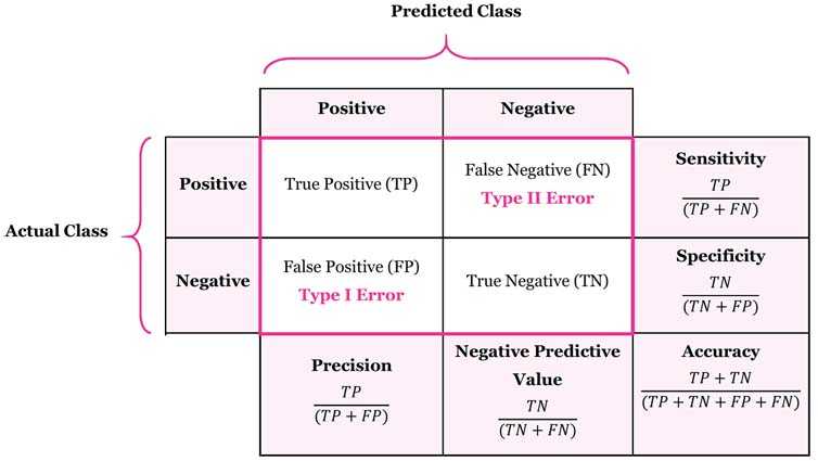
Confusion Matrix

Actual	Predicted-No	Predicted-Yes
No	True Negatives	False Positives
Yes	False Negatives	True Positives

from sklearn import metrics confusion = metrics.confusion_matrix(y_train_pred_final.Churn, y_train_pred_final.predicted ) TP = confusion[1,1] # true positive TN = confusion[0,0] # true negatives FP = confusion[0,1] # false positives FN = confusion[1,0] # false negatives

Accuracy

$Accuracy = \frac{True\;Negative + True\;Positive}{Total\;Negative + Total\;Positive}$

Sensitivity

$Sensitivity = \frac{Number\;of\;actual\;YESes\;correctly\;predicted}{Total\;number\;of\;actual\;YESes} = \frac{TP}{TP+FN}$

• This is also called as True Positive Rate
• This is also called signal
• We want to maximise this ratio

Specificity

$Specificity = \frac{Number\;of\;actual\;NOs\;correctly\;predicted}{Total\;number\;of\;actual\;Nos} = \frac{TN}{TN + FP}$

False Positive Rate

$False\;Positive\;Rate = \frac{False\;Positive}{True\;Negative+False\;Positive} = \frac{FP}{TN+FP}$

• This is same as (1 - Specificity)
• This is also called Noise
• We want to minimise this ratio

Negative Predictive Value

$Negative\;Predictive\;Value = \frac{True\;Negative}{True\;Negative + False\;Negative} = \frac{TN}{TN+FN}$

Positive Predictive Value

• This is also know as Precision $Precision = \frac{TP}{TP+FP}$

Receiver Operating Characteristic Curve - ROC Curve

• Plot between False Positive Rate (x-axis) and True Positive Rate (y-axis) is termed as the ROC curve.
• It shows the trade-off between sensitivity and specificity
• It will always start at (0,0) and end at (1,1)
• When the value of TPR (on the Y-axis) is increasing, the value of FPR (on the X-axis) also increases.
• Model should have Low FPR and High TPR
• A good ROC curve is the one which touches the upper-left corner of the graph. The AUC will be higher for such a curve.
• The closer the curve comes to the 45-degree diagonal of the ROC space, the less accurate the test. The AUC will be lower for such a curve.
• Higher the area under the curve (AUC) of an ROC curve, the better is your model
• The least area of ROC curve is 0.5 (x=y)
• The highest area of ROC curve is 1 (y=1, x={0,1})
• If there are spikes in the ROC curve, it means that the model is not stable

• As can be seen from the graph, better the classification (i.e. higher separation between classes), higher the AUC.

def draw_roc( actual, probs ): fpr, tpr, thresholds = metrics.roc_curve( actual, probs, drop_intermediate = False ) auc_score = metrics.roc_auc_score( actual, probs ) plt.figure(figsize=(5, 5)) plt.plot( fpr, tpr, label='ROC curve (area = %0.2f)' % auc_score ) plt.plot([0, 1], [0, 1], 'k--') plt.xlim([0.0, 1.0]) plt.ylim([0.0, 1.05]) plt.xlabel('False Positive Rate or [1 - True Negative Rate]') plt.ylabel('True Positive Rate') plt.title('Receiver operating characteristic example') plt.legend(loc="lower right") plt.show() return None # Calling the function draw_roc(y_train_pred_final.Churn, y_train_pred_final.Churn_Prob)

---

Questions

Q: Given the ROC curves of 3 models A, B & C, which model is the best?

• The Area under Curve for C is the largest, hence it is the best model among the three.

---

Q: Let's say that you are building a telecom churn prediction model with the business objective that your company wants to implement an aggressive customer retention campaign to retain the 'high churn-risk' customers. This is because a competitor has launched extremely low-cost mobile plans, and you want to avoid churn as much as possible by providing incentives to the customers. Assume that budget is not a constraint. Which of Sensitivity, Specificity, and Accuracy will you choose to maximise?

• Sensitivity: high sensitivity implies that your model will correctly identify almost all customers who are likely to churn. It will do that by over-estimating the churn likelihood, i.e. it will misclassify some non-churns as churns, but that is the trade-off we need to choose rather than the opposite case (in which case we may lose some low churn risk customers to the competition).

Precision

• $Precision = \frac{TP}{TP+FP}$
• probability that a predicted 'yes' is actually 'yes'
• formula is same as Positive Predicted Value
• The curve for precision can be jumpy because the denominator is not constant, it changes based on the threshold

from sklearn import metrics metrics.precision_score(y_train, y_pred)

Recall

$Recall = \frac{TP}{TP+FN}$

• probability that 'yes' case is predicted as such
• formula is same as True Positive Ratio / Sensitivity
• detection rate

from sklearn import metrics metrics.recall_score(y_train, y_pred)

Note: Increase Precision => Decrease Recall and vice-versa

---

Questions

Q: Calculate F1-Score given the confusion matrix below

Actual / Predicted	Not Churn	Churn
Not Churn	400	100
Churn	50	150

• F1-Score is the harmonic mean of precision and recall
• $F = 2 * \frac{(precision*recall)}{(precision + recall)}$
• $Precision = \frac{TP}{TP+FP} = \frac{150}{150+100} \approx 0.66$
• $Recall = \frac{TP}{TP+FN} = \frac{150}{150+50} \approx 0.75$
• $F = 2*\frac{0.6*0.75}{0.6+0.75} \approx 0.67$

---

Summary - Steps of Building a Classification Model

1. Data cleaning and preparation

   • Combining dataframes
   • Handling categorical variables
   • Mapping categorical variables to integers
   • Dummy variable creation
   • Handling missing values
2. Test-train split and scaling

3. Model Building

   • Feature elimination based on correlations
   • Feature selection using RFE (Coarse Tuning)
   • Manual feature elimination (using p-values and VIFs)

4. Model Evaluation

   • Accuracy
   • Sensitivity and Specificity
   • Optimal cut-off using ROC curve
   • Precision and Recall
5. Predictions on the test set

Takeaways

• There is a trade off between TPR and FPR or Sensitivity and Specificity
• When building a Logistic Regression model, we will perform the steps of data cleaning, EDA, Feature Selection, train-test split, scaling. These are steps that are to be performed for any model.
• In Classification Models, we should look at statistics such as Specificity, Sensitivity, Precision and Recall. As per business understanding, we may have to prefer one metric over the other. Generally, the optimal cut off will be the one where the values for specificity, and sensitivity are similar.
• Precision-Recall and Specificity-Sensitivity are two views of the same problem and the choice depends on the business.

Measures of Discriminative Power

Sheet Demonstrating Gain, Lift and KS Statistic

• Note: Download this file as an excel to view the charts properly

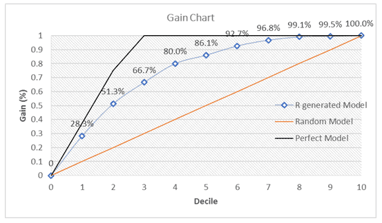
Gain

• Create a model
• Sort by probability of churn
• Create buckets
• Findd cumulative probability
• Generate Gain Chart

Lift

• Create a Random Model
• Compare random model vs our model
• Lift tells you the factor by which your model is outperforming a random model, i.e. a model-less situation
• Formula: $\displaystyle \frac{\text{Gain for Current Model}}{\text{Gain for Random Model}}$

KS Statistic

• The KS statistic is an indicator of how well your model discriminates between the two classes.
• The KS statistic gives you an indicator of where you lie between the random and perfect model

• A good model will be such that:

  • \ge 40% KS Statistic
  • lies in the top deciles, i.e. 1st, 2nd, 3rd or 4th
• It is caclualated as {% cumulative churn - % cumulative non-churn} for every decile

References

• https://www.mathplanet.com/education/algebra-1/exponents-and-exponential-functions/properties-of-exponents
• https://www.mathplanet.com/education/algebra-2/exponential-and-logarithmic-functions/logarithm-property
• https://www.rapidtables.com/math/algebra/Logarithm.html
• https://www.khanacademy.org/math/algebra2/x2ec2f6f830c9fb89:logs/x2ec2f6f830c9fb89:log-intro/v/logarithms?modal=1
• https://datascience.stackexchange.com/questions/12321/whats-the-difference-between-fit-and-fit-transform-in-scikit-learn-models
• https://towardsdatascience.com/receiver-operating-characteristic-curves-demystified-in-python-bd531a4364d0
• https://en.wikipedia.org/wiki/Harmonic_mean