• Recurrent Neural Networks
• What are Sequences
• RNN Formulation

• Architecture of RNN

  • The flow of information in RNNs is as follows
  • Example
  • Unrolled RNN
  • Rolled RNN

• Feeding Sequences to RNNs

  • IID Data - Independently and Identically Distributed Data
  • Question
• Sizes of Components of RNN
• RNNs: Simplified Notations

• Trainable Parameters

  • Output Layer
  • RNN Unit Connections
  • Formula for Number of Parameters
  • Question

• Types of RNNs

  • Many-to-one RNN
  • Loss
  • Many-to-many RNN: Equal input and output length
  • Many-to-many RNN: Unequal input and output lengths
  • Loss
  • One-to-many RNN
• Loss
• Quesions
• The Gradient Propagation Problem in RNNs
• Questions

Recurrent Neural Networks

• RNNs are specially designed to work with sequential data, i.e. data where there is a natural notion of a 'sequence' such as text (sequences of words, sentences etc.), videos (sequences of images), speech etc.
• RNNs have been able to produce state-of-the-art results in fields such as natural language processing, computer vision, and time series analysis.
• One particular domain RNNs have revolutionised is natural language processing.
• RNNs have given, and continue to give, state-of-the-art results in areas such as machine translation, sentiment analysis, question answering systems, speech recognition, text summarization, text generation, conversational agents, handwriting analysis and numerous other areas.
• In computer vision, RNNs are being used in tandem with CNNs in applications such as image and video processing.
• Many RNN-based applications have already penetrated consumer products. Take, for example, the auto-reply feature which you see in many chat applications, as shown below:

LinkedIn Auto Reply

GMail Auto Reply

You may have noticed auto-generated subtitles on YouTube (and that it has surprisingly good accuracy). This is an example of automatic speech recognition (ASR) which is built using RNNs.

• RNNs are also being used in applications other than NLP.
• Recently, OpenAI, a non-profit artificial intelligence research company came really close to defeating the world champions of Dota 2, a popular and complex battle arena game.
• The game was played between a team of five bots (from OpenAI) and a team of five players (world champions).
• The bots were trained using reinforcement learning and recurrent neural networks.
• There are various companies who are generating music using RNNs. AIVA is one such company.
• There are many other problems which are yet to be solved, and RNNs look like a promising candidate to solve them.

What are Sequences

Just like CNNs were specially designed to process images, Recurrent Neural Networks (RNNs) are specially designed to process sequential data.

In sequential data, entities occur in a particular order. If you break the order, you don’t have a meaningful sequence anymore. For example,

• you could have a sequence of words which makes up a document. If you jumble the words, you will end up having a nonsensical document.
• Similarly, you could have a sequence of images which makes up a video. If you shuffle the frames, you’ll end up having a different video.
• Likewise, you could have a piece of music which comprises of a sequence of notes. If you change the notes, you’ll mess up the melody.

Recurrent neural networks are variants of the vanilla neural networks which are tailored to learn sequential patterns.

Normal Neural Networks can approximate any given function, while Recurrent Neural Networks can simulate any given algorithm

The state of the recurrent network updates itself as it sees new elements in the sequence. This is the core idea of an RNN - it updates what it has learnt as it sees new inputs in the sequence. The 'next state' is influenced by the previous one, and so it can learn the dependence between the subsequent states which is a characteristic of sequence problems.

RNN Formulation

The most basic form can be expressed as:

$a_{t+1}^{(l)} = g(a_{t}^{(l)}, z_{t+1}^{(l)})$

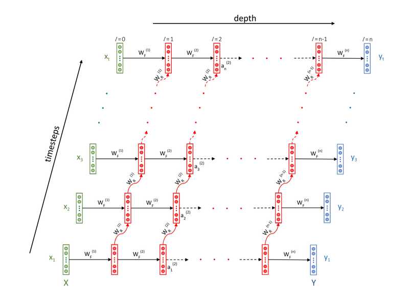
• The main different between normal neural nets and RNNs is that RNNs have two 'dimensions' - time $t$ (i.e. along the sequence length) and the depth $l$ (the usual layers).
• The basic notation itself changes from $a^l$ to $a^l_t$.
• In fact, in RNNs it is somewhat incomplete to say 'the output at layer $l$'; we rather say 'the output at layer $l$ and time $t$'
• One way to think about RNNs is that the network changes its state with time (as it sees new words in a sentence, new frames in a video etc.).

• The output of layer $l$ at time $t+1$, $a^l_{t+1}$, depends on two things:

  1. The output of the previous layer at the same time step $a_{t+1}^{l+1}$ (this is the depth dimension).
  2. Its own previous state $a_t^l$ (this is the time dimension)

In other words, $a^l_{t+1}$ is a function of $a_{t+1}^{l-1}$ and $a_t^l$:
$a_{t+1}^{(l)} = g(a_{t}^{(l)}, z_{t+1}^{(l)})$

We say that there is a recurrent relationship between $a^l_{t+1}$ and its previous state $a^l_t$, and hence the name Recurrent Neural Networks.

The feedforward equations are extensions of the vanilla neural nets - the only difference being that now there is a weight associated with both $a_{t+1}^{l+1}\; \text{and}\; a^l_t$.

$a^l_{t+1} = \sigma(W_F.a^{l-1}_{t+1} + W_R.a^l_t + b^l)$

The $W_F$'s are called the feedforward weights and the $W_R$'s are called the recurrent weights.

Architecture of RNN

• The green layer is the input layer in which the $x_i$'s are elements in a sequence - words of a sentence, frames of a video, etc.
• The layers in red are the 'recurrent layers' - they represent the various states evolving over time as new inputs are seen by the network.
• The blue layer is the output layer where the $y_i$'s are the outputs emitted by the network at each time step.

For example, in a parts of speech (POS) tagging task (assigning tags such as noun, verb, adjective etc. to each word in a sentence), the $yi$'s will be the POS tags of the corresponding $x_{i}$'s.

Note that in this figure, the input and output sequences are of equal lengths, but this is not necessary. For e.g. to classify a sentence as 'positive/negative' (sentiment-wise), the output layer will emit just one label (0/1) at the end of T timesteps

You can see that the layers of an RNN are similar to the vanilla neural nets (MLPs) - each layer has some neurons and is interconnected to the previous and the next layers. The only difference is that now each layer has a copy of itself along the time dimension (the various states of a layer, shown in red colour). Thus, the layers along the time dimension have the same number of neurons (since they represent the various states of same $l_{th}$ layer over time).

The flow of information in RNNs is as follows

• each layer gets the input from two directions

  • activations from the previous layer at the current timestep and
  • activations from the current layer at the previous timestep.

• Similarly, the activations (outputs from each layer) go in two directions

  • towards the next layer at the current timestep (through $W_F$), and
  • towards the next timestep in the same layer (through $W_R$).
• The 'depth' of an RNN refers to the number of layers in the RNN
• All the timesteps at a particular layer are virtual copies of the same layer. The only difference between different timesteps at a particular layer is their state.

Example

The inputs going into the second layer at the 8th time step are:

• $a^1_8$: output from previous layer at current timestep
• $a^2_7$: output from current layer at previous timestep

The following outputs (activations) will necessarily have the same size:

• $a^4_3, a^4_5$, $a^2_2, a^2_6$
• This is because same layers are copied over at different timesteps
• The outputs of any layer at different steps will be of exactly the same size since they basically represent the output of the same layer evolving over time.

However, the same cannot be said for

• $a^4_3, a^3_5$, $a^2_2, a^3_6$
• Since different layers (at each depth) can have different number of neurons

Unrolled RNN

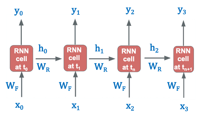
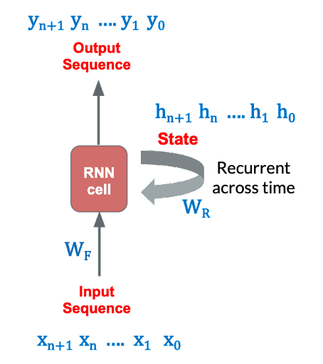
In the diagram given below, the input $(x_t)$ and hidden state $(h_t)$ are shown at each time step t, which are changing across time steps. Both $x_t$ and $h_t$ have their separate weights $W_F$ and $W_R$ respectively, which remain the same for each time step as depicted by just using $W_F$ and $W_R$ at each time step.

Rolled RNN

Feeding Sequences to RNNs

• In the case of an RNN, each data point is a sequence.
• The individual sequences are assumed to be independently and identically distributed (I.I.D.), though the entities within a sequence may have a dependence on each other.
• As the network keeps ingesting new elements in the sequence it updates its current state (i.e. updates its activations after consuming each element in the sequence).
• After the sequence is finished (say after T time steps), the output from the last layer of the network $a_T^L$ captures the representation of the entire sequence.
• You can now do whatever you want with this output - use it to classify the sentence as correct/incorrect, feed it to a regression output, etc.
• This is exactly analogous to the way CNNs are used to learn a representation of images, and one can use those representations for a variety of tasks.

IID Data - Independently and Identically Distributed Data

• In a sentence classification task (grammatically correct/incorrect), the individual sentences used for training are IID
• In a video classification task (contains violence/does not contain violence), the individual videos are IID

Question

Consider a batch of 50 sequences. Suppose you have trained an RNN model with these sequences. Let’s call this model A. Now, suppose you want to train another model B which has the exact same architecture as model A. Assume that the training is not stochastic in nature (that is, all the seed values are same while initialising the network parameters). Which of the following actions will result in a different set of weights for model B after the training is done in the exact same fashion as done in case of model A?

Statement	True / False
Shuffling the order of entities within each sequence.	True
Shuffling the order of the sequences in the training data.	False

• Since entities within a sequence are dependent on each other, changing the sequence will result in a different sequence altogether.
• This will result in the RNN learning a different representation for the sequence and model B would eventually end up having different set of weights than model A.

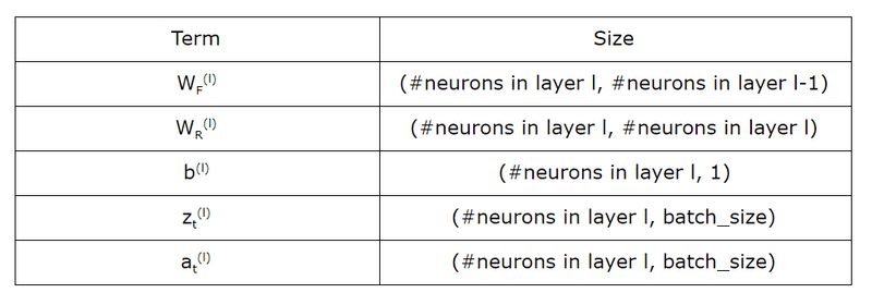
Sizes of Components of RNN

RNNs: Simplified Notations

The RNN Feedforward equations are:

• $z^t_t = W^l_Fa^{l-1}_t + W^l_Ra^{l}_{t-1} + b^l$
• $a^l_t = f^l(z^l_t)$

The above equation can be written in the following matrix form:

• $z_t^l = \begin{bmatrix}W^l_F & W^l_R\end{bmatrix}\begin{bmatrix}a^{l-1}_t \\ a^l_{t-1}\end{bmatrix}+b^l$

We can now merge the two weight matrices into one to get the following notation:

• $z^l_t = W^l\begin{bmatrix}a_t^{l-1}, a_{t-1}^l\end{bmatrix} + b^l$

where $W^l$ denotes the feedforward + recurrent weights of layer $l$ formed by stacking (or concatenating) $W^l_F$ and $W_R^l$ side by side and $\begin{bmatrix}a^{l-1}_t,a^l_{t-1}\end{bmatrix}$ on top of each other.

This form is not only more concise but also more computationally efficient. Rather than doing two matrix multiplications and adding them, the network can do one large matrix multiplication.

Trainable Parameters

Output Layer

• There is a dense connection between output layer and RNN Layer
• Number of output layer weights = Number of RNN units * Number of output nodes
• Number of biases = Number of output nodes

RNN Unit Connections

• The hidden RNN layer constitutes connections across each of the RNN units as each of these units needs to know what is going inside the other unit for efficient results.

Formula for Number of Parameters

Configurable parameters of a Simple RNN Layer

• No of Simple RNN units in a layer
• No of input streams fed into the network, acting as features

Parameters for different Layers

• Number of Input Weights = Number of input features * Number of RNN Units
• Number of Recurrent Weights = Number of RNN units * Number of RNN Units
• Number of Biases = Number of RNN Units

Total Parameters

• Total trainable parameters = Number of Input Weights + Number of Recurrent Weights + Number of Biases = (numfeatures*numunits)+(numunits*numunits)+num_units

Question

Assuming we have an RNN network with 4 input features, then 5 RNN units and then 3 output labels.

• Number of Input Weights = 4*5 = 20
• Number of Recurrent Weights = 5*5 = 25
• Number of Biases = Number of RNN Units = 5
• Number of Output Layer Weights = 5*3 = 15
• Number of Biases = Number of Output Nodes = 3
• Total Parameters = input parameters + recurrent parameters + output parameters = 20 + (25+5) + (15+3) = 68

Just like the ANNs, the dimensions of the weights and biases in RNNs will be dependent upon the number of input features, number of hidden RNN units and number of output nodes. In the network we used above, considering that each input will be a single numeric value hence overall dimensions (1x4), the input weights will be of dimension (4x5). Similarly the recurrent weights will have dimensions (5x5), the recurrent bias (1x5) and Output weight will be a matrix of dimension (5x3).

Types of RNNs

Many-to-one RNN

In this architecture, the input is a sequence while the output is a single element. We have already discussed an example of this type - classifying a sentence as grammatically correct/incorrect. The figure below shows the many-to-one architecture:

Note that each element of the input sequence $x_{i}$ is a numeric vector. For words in a sentence, you can use a one-hot encoded representation, use word embeddings etc.

Some other examples of many-to-one problems are:

• Predicting the sentiment score of a text (between -1 to 1). For e.g., you can train an RNN to assign sentiment scores to customer reviews etc. Note that this can be framed as either a regression problem (where the output is a continuous number) or a classification problem (e.g. when the sentiment is positive/neutral/negative)
• Classifying videos into categories. For example, say you want to classify YouTube videos into two categories 'contains violent content / does not contain violence'. The output can be a single softmax neuron which predicts the probability that a video is violent.

Here, at the last layer, we only care about the activation coming from the last timestep i.e. activation after the full sequence has been pushed through the network.

Loss

In a many-to-one architecture (such as classifying a sentence as correct/incorrect), the loss is simply the difference between the predicted and the actual label. The loss is computed and backpropagated after the entire sequence has been digested by the network.

Many-to-many RNN: Equal input and output length

In this type of RNN, the input (X) and output (Y) both are a sequence of multiple entities spread over timesteps.

In this architecture, the network spits out an output at each timestep. There is a one-to-one correspondence between the input and output at each timestep. You can use this architecture for various tasks.

Example: Part of Speech Tagger

Many-to-many RNN: Unequal input and output lengths

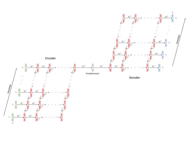
In the previous many-to-many example of POS tagging, we had assumed that the lengths of the input and output sequences are equal. However, this is not always the case. There are many problems where the lengths of the input and output sequences are different. For example, consider the task of machine translation - the length of a Hindi sentence can be different from the corresponding English sentence.

The encoder-decoder architecture is used in tasks where the input and output sequences are of different lengths.

The above architecture comprises of two components - an encoder and a decoder both of which are RNNs themselves. The output of the encoder, called the encoded vector (and sometimes also the 'context vector'), captures a representation of the input sequence. The encoded vector is then fed to the decoder RNN which produces the output sequence.

You can see that the input and output can now be of different lengths since there is no one-to-one correspondence between them anymore. This architecture gives the RNNs much-needed flexibility for real-world applications such as language translation.

Loss

In a many-to-many architecture, the network emits an output at multiple time steps, and the loss is calculated at each time step. The total loss (= the sum of the losses at each time step) is propagated back into the network after the entire sequence has been ingested.

In encoder-decoder architecture,

• The loss is backpropagated to the encoder through the decoder. Backpropagation starts from the output sequence of the decoder and ends at the input sequence.
• The loss is calculated after every timestep of a sequence.
• The loss corresponding to each element of the output sequence can be computed as they are being produced by the decoder. The loss corresponding to each output element can be computed on the fly as the outputs are being emitted by the decoder layer. They are added to get the total loss after all the time steps are over.
• The loss is backpropagated after the entire sequence (or a batch of sequences) has been ingested by the network. Backpropagation only starts when the total loss of a sequence is computed (in fact, only after the total loss for a batch of sequences is computed).
• The total loss of a sequence is the sum of the losses of the individual output elements of the sequence

One-to-many RNN

In this type of RNN, the input is a single entity, and output consists of a sequence. The following image shows such an architecture:

This architecture hasn't been used in the fields of computer vision or natural language processing. Rather, it has been used by a wide variety of industries such as music and arts.

This type of architecture is generally used as a generative model. Among popular use of this architecture are applications such as generating music (given a genre, for example), generating landscape images given a keyword, generating text given an instruction/topic, etc.

Loss

• Let the network have $T_1$ input time steps and $T_2$ output time steps.
• The input-output pairs are thus $(x_1, x_2, \ldots, x_{T_1})$ and $(y_1, y_2, \ldots, y_{T_2})$
• $T_1$ and $T_2$ can be unequal.

In many-to-one architectures, the output length $T_2=1$, i.e. there is only a single output $y_{out}$ for each sequence. If the actual correct label of the sequence is $y$, then the loss $L$ for each sequence is (assuming a cross-entropy loss):

$L = \text{cross-entropy}(y_{out}, y)$

In a many-to-many architecture, if the actual output is $(y_1, y_2, \ldots, y_{T_2})$ and the predicted output is $(y_1', y_2', ..., y'_{T_2})$, then the loss $L$ for each sequence is:

$l = \sum_{i=1}^{T_2}\text{cross-entropy}(y_{i}', y_{i}')$

We can now add the losses for all the sequences (i.e. for a batch of input sequences) and backpropagate the total loss into the network.

Quesions

Suppose you have a corpus of English documents along with the summary of each document. You want to train an RNN model to build a document summarizer. Which of the following architectures is suited best for this problem?

• The input comprises of a sequence, the document, which is greater in length than the length of the output sequence, the summary. Therefore an encoder-decoder architecture will be the most suitable of all the enlisted ones.

Let’s say you want to predict whether a person will click on an advertisement link based on features such as browsing time on the website, timestamp, gender, age, occupation, ethnicity, etc. Which of the following RNN architectures will be most suitable for this kind of problem?

• The problem is doesn't involve any sequences. Therefore, an RNN won’t be suitable for this type of problem. A standard feedforward network more appropriate in this case.

Let’s say you’re working for a company which wants to build an AI keyboard for smartphones. The aim of the company is to build such a keyboard which predicts the next word based on previous few words that the user has typed. For example, when someone types "Hey, I will be late to the ___", the network should predict the next word (say) "office".

• The input is a sequence of words based on which the next word, a single entity, will be predicted. Hence, a many-to-one architecture will be most suitable in this case.

Suppose you’re working for an online video streaming company that wants to caption each frame of the videos with the actor name that is present in each scene. What architecture do you think would be most suitable for this job?

• The input is a video, which is nothing but a sequence of images, and the output is the actor’s name in the scene. Hence a standard many-to-many architecture will be suitable for this problem.

The Gradient Propagation Problem in RNNs

• Although RNNs are extremely versatile and can (theoretically) learn extremely complex functions, the biggest problem is that they are extremely hard to train (especially when the sequences get very long).
• RNNs are designed to learn patterns in sequential data, i.e. patterns across 'time'. RNNs are also capable of learning what are called long-term dependencies. For example, in a machine translation task, we expect the network to learn the interdependencies between the first and the eighth word, learn the grammar of the languages, etc. This is accomplished through the recurrent layers of the net - each state learns the cumulative knowledge of the sequence seen so far by the network.
• Although this feature is what makes RNNs so powerful, it introduces a severe problem - as the sequences become longer, it becomes much harder to backpropagate the errors back into the network. The gradients 'die out' by the time they reach the initial time steps during backpropagation.
• RNNs use a slightly modified version of backpropagation to update the weights. In a standard neural network, the errors are propagated from the output layer to the input layer. However, in RNNs, errors are propagated not only from right to left but also through the time axis.

• Refer to the figure above - notice that the output $y_t$ is not only dependent on the input $x_t$, but also on the inputs $x_{t-1}, x_{t-2}$, and so on till $x_1$. Thus, the loss at time $t$ depends on all the inputs and weights that appear before $t$. For e.g. if you change $W_F^2$, it will affect all the outputs $a_1^2, a_2^2, a_3^2$, which will eventually affect the output $y_t$ 9through a long feedforward chain).
• This implies that the gradient of the loss at time $t$ needs to be propagated backwards through all the layers and all the time steps. To appreciate the complexity of this task, consider a typical speech recognition task - a typical spoken English sentence may have 30-40 words, so you have to backpropagate the gradients through 40 time steps and the different layers.
• This type of backpropagation is known as backpropagation through time or BPTT.

• The exact backpropagation equations are covered in the optional session, though here let's just understand the high-level intuition. The feedforward equation is:

  $a_t^1 = f(W_F^la_t^{l-1} + W_R^la^l_{t-1} + b^l)$

• Now, recall that in backpropagation we compute the gradient of subsequent layers with respect to the previous layers. In the time dimension, we compute the gradient of output at time $t$ with respect to the output at $t-1$, i.e. $\frac{\partial a^l_t}{\partial a^l_{t-1}}$. This quantity depends linearly on $W_R$, so $\frac{\partial a_t^l}{\partial a_{t-1}^l}$ is some function of $W_R$:

  $\frac{\partial a_t^l}{\partial a^l_{t-1}} = g(W_R)$

• Similarly, extending the gradient one time step backwards, the gradient $\frac{\partial a^l_{t-1}}{\partial a^l_{t-2}}$ will also be a function of $W_R$, and so on. The problem is that these gradients are eventually multiplied with each other during backpropagating, and so the matrix $W_R$ is raised to higher and higher power of its own, $(W_R)^n$, as the error propagates backwards in time.
• The longer the sequence, the higher the power. This leads to exploding or vanishing gradients. If the individual entries of $W_R$ are greater than one, the values in $(W_R)^n$ will explode to extremely large values; if the entries are lesser than one, $(W_R)^n$ will make them extremely small.
• You could still use some workarounds to solve the problem of exploding gradients. You can impose an upper limit to the gradient while training, commonly known as gradient clipping. By controlling the maximum value of a gradient, you could do away with the problem of exploding gradients.
• But the problem of vanishing gradients is a more serious one. The vanishing gradient problem is so rampant and serious in the case of RNNs that it renders RNNs useless in practical applications. One way to get rid of this problem is to use short sequences instead of long sequences. But this is more of a compromise than a solution - it restricts the applications where RNNs can be used.
• To get rid of the vanishing gradient problem, researchers have been tinkering around with the RNN architecture for a long while. The most notable and popular modifications are the long short-term memory units (LSTMs) and the gated recurrent units (GRUs).

Questions

While backpropagating, one is supposed to calculate the gradient of the loss w.r.t. the weights sitting at different layers. While backpropagating, which of the following entities will have an influence on the gradient of $y_3$?

• $x_1, x_2, and x_3$
• $y_3$ will depend on each input till $x_3$

Which of the following techniques will have no effect on the either of the two problems: vanishing and the exploding gradients?

Statement	True / False
Making the sequence longer or shorter	False
Putting an upper limit to the gradient by clipping it	False
Changing the architecture from many-to-many to many-to-one	True

• Changing the architectures will have no effect in the architecture as far as calculations are concerned. The vanishing and exploding gradients problem is because of sequence length, not because of the type of architecture in use.

Suppose you’re building a sentiment classifier based on users’ reviews on a product. The model is expected to predict a numeric ‘sentiment score’ for each review. Which of the following RNN architectures will be most suitable for this kind of problem?

• Many-to-one architecture
• The input, a review, is a sequence of words and the output, the sentiment label, is a single entity. Hence, this architecture will be most suitable in this case.

Consider a many-to-one recurrent neural network with 20 timesteps and a batch size of 32 (batch size refers to the number of sequences fed into the network in one iteration). The network architecture is as follows:

What is the size of $W_R^2$?

• (8, 8)
• We know that the $W^l_R$ is of size (#neurons at layer l, #neurons at layer l). The second hidden layer has 8 neurons. Therefore, its dimension is (8, 8).

What is the size of $a^1_8$?

• (5, 32)
• We know that the size of $a^l_t$ is (#neurons at layer l, #batch_size). The first hidden layer has 5 neurons and the batch size is 32. Therefore, its dimension is (5, 32).

What of the following statement is incorrect?

Statement	True / False
The size of $W^1_F$ is greater than the size of $W^1_R$	False
The activations at the output layer consist of a vector of 32 elements	False
The size of $a^2_3$ is larger than the size of $a^2_{10}$.	True. Size of both $a_3^2$ and $a^2_{10}$ is (8, 32).
The bias of the output layer $b^3$ is equivalent to a scalar	False

Suppose you change the batch size from 32 to 128. Which of the following matrix sizes will be affected by this change?

• $a^2_{20}$
• The size of $a^2_20$ will change to (8, 128) from (8, 32) after changing the batch size.