• Support Vector Machines
• Maximal Marginal Classifier
• Soft Margin Classifier
• Summary
• Questions
• Kernels

• Boundary Transformation

  • Feature Transformation

• How Kernls Work

  • The Kernel Trick

  • Practical Considerations

    • Hyperparameters in Non Linear Kernels
• Questions
• Applications of SVMs

Support Vector Machines

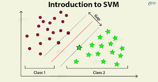
• These are models that help in separating points into different classes by creating hyperplanes.
• The hyperplanes are high dimensional planes that are hard to visualize but can be expressed using simple a simple equation: $ax_1 + bx_2 + cx_3 + dx_4 + constant = 0$ and so on.
• Any point whose value is greater than 0 (when put into the hyperplane equation) belongs to class one, while any point below will be marked as class two.
• Any point that is equal to zero will lie perfectly on the hyperplane
• SVMs create planes such that the closest points of both classes from the hyperplane have equal distance. In other words, they create a margin so as to give some breathing room for both points to lie in a specified region.
• The SVMs are defined by the support vectors. Support Vectors are vectors formed on either side of the hyperplane using the closing points described in the previous point.

Maximal Marginal Classifier

• It is a hard classifier

• The equation for the plane can be written as: $l.\overrightarrow{w}\overrightarrow{y} \ge 0$; where

  • l is the label (-1/1)
  • w is the weights vector
  • y is the data points vectors
• We rescale the values of w such that the weights are normalized to write the equation in the above form.

Soft Margin Classifier

The mathematical formulation for the Maximal Margin Classifier can be expressed as: $\displaystyle l_{i}X(W.Y_{i})\ge M$ where

• $l_{i}$ represents the label of the ith observation (such as spam(+1) and ham(-1));
• W represents the vector of the coefficients (or weights) of each attribute (for example, if you have 3 attributes, W = [w0, w1, w2, w3]).
• $Y_{i}$ represents the vector of the attribute values for the ith row, e.g. Y = [1,y1, y2, y3] for 3 attributes.

Thus, the dot product $W.Y_{i}$ is simply the value of the expression obtained by putting the ith data point in the hyperplane equation, i.e. $w_0 + w_1y_1 + r_2y_2 + w_3y_3$.

Thus, $W.Y_{i}$ is lesser than, equal to or greater than 0, depending on the location of the ith data point with respect to the hyperplane. Also, note that the value of $W.Y_{i}$ gives you the distance of the ith data point from the hyperplane.

• M represents the margin, i.e. the distance of the closest data point from the hyperplane.

If you impose the condition $\displaystyle l_{i}X(W.Y_{i})\ge M$ on the model, then you are implying that you want each point to be at least a distance M away from the hyperplane. But unfortunately, few real datasets will be so easily, perfectly separable. Thus, to relax the constraint, you include a ‘slack variable’ \epsilon_i for each data point i.

Thus, you modify the formulation to $\displaystyle l_{i}X(W.Y_{i})\ge M(1-\epsilon_i)$, where the slack variable ($\epsilon_i$) takes a value between 0 to infinity.

Depending on the value of $\epsilon_i$, the ith data point can now take any position - it can fall on the correct side of the margin (and a safe distance away), or inside the margin (but still correctly classified), or even stray on the wrong side of the hyperplane itself.

Summary

• Maximal Margin Classifier has certain limitations. It will not find a separator if the classes are not linearly separable (as shown below).
• The Soft Margin Classifier overcomes the drawbacks of the Maximal Margin Classifier by allowing certain points to be misclassified.
• You control the amount of misclassifications using the cost of misclassification 'C', where C is the maximum value of the summation of the slack variable epsilon(ϵ), i.e. $\sum \epsilon_i \le C$.
• If C is high, a higher number of points are allowed to be misclassified or violate the margin. In this case, the model is flexible, more generalisable, and less likely to overfit. In other words, it has a high bias.
• On the other hand, if C is low, a lesser numer of points are allowed to be misclassified or violate the margin. In this case, the model is less flexible, less generalisable, and more likely to overfit. In other words, it has a high variance.
• So, C represents the 'liberty of misclassification' that you provide to the model.
• Note that the C defined above and the parameter C used in the SVC() function in python are the inverse of each other. In SVC(), C represents the 'penalty for misclassification'.

Questions

The data points on the edge of the ‘band’, around the separator that makes all the data points outside the band redundant, are called

• Support vectors: Support vectors are the data points that lie close to the Support Vector Classifier; they are the only data points used for constructing the classifier.

For two classes, i.e. class A and class B, If the number of data points that are misclassified is more for class A than that for class B, then for a cost-sensitive SVM model, decreasing the value of C should

• Shift the separator towards class B: According to SVM formulation, if C has a high value, it will allow misclassifications. However, a low value of C will not allow any points to be misclassified. So with the cost being high for class A, the separator would be shifted towards B.

---

Kernels

• Kernels are one of the most interesting inventions in machine learning, partly because they were born through the creative imagination of mathematicians, and partly because of their utility in dealing with non-linear datasets.
• Many real-world data sets are not separable by linear boundaries. For instance, what if the distribution of data points looks like the figure given below?

• You’ll agree that it is not possible to imagine a linear hyperplane (a line in 2D) that separates the red and blue points reasonably well. Thus, you need to tweak the linear SVM model and enable it to incorporate nonlinearity in some way.
• Kernels serve this purpose — they enable the linear SVM model to separate nonlinearly separable data points.
• It is important to remember that SVMs are linear models, and kernels do not change this at all. Kernels are ‘toppings’ over the linear SVM model, which somehow enable the model to separate nonlinear data.

Boundary Transformation

You can transform nonlinear boundaries to linear boundaries by applying certain functions to the original attributes. The original space (X, Y) is called the original attribute space, and the transformed space (X’, Y’) is called the feature space.

Ex: Equation of an Ellipse

• $\frac{x^{2}}{a}+\frac{y^{2}}{b} = c$

Feature Transformation

• There is an exponential increase in the number of dimensions when you transform the attribute space to a feature space. This makes the modelling (i.e. the learning process) computationally expensive.

Ex: Quadratic

• x, y $\rightarrow$ x, y, xy, x^2, y^2, c

How Kernls Work

• Kernels are like black boxes where the original attributes are passed and it spits out the transformed attributes in a higher dimensional feature space. The SVM algorithm is shown only the transformed, linear feature space, where it builds the linear classifier as usual

• However, what makes kernels special is that they don't do this transformation explicitly (which is a computationally difficult task), but they use a mathematical hack to do this implicitly.

The Kernel Trick

• The key fact that makes the kernel trick possible is that to find a best fit model, the learning algorithm only needs the inner products of the observations ($X^T_i.Xj$). It never uses the individual data points X1, X2 etc. in silo.

• Kernel functions use this fact to bypass the explicit transformation process from the attribute space to the feature space, and rather do it implicitly. The benefit of implicit transformation is that now you do not need to:

  • Manually find the mathematical transformation needed to convert a nonlinear to a linear feature space
  • Perform computationally heavy transformations

Practical Considerations

In practice, you only need to know that kernels are functions which help you transform non-linear datasets. Given a dataset, you can try various kernels, and choose the one that produces the best model. The three most popular types of kernel functions are:

1. The linear kernel: This is the same as the support vector classifier, or the hyperplane, without any transformation at all

2. The polynomial kernel: It is capable of creating nonlinear, polynomial decision boundaries

3. The radial basis function (RBF) kernel: This is the most complex one, which is capable of transforming highly nonlinear feature spaces to linear ones. It is even capable of creating elliptical (i.e. enclosed) decision boundaries

Hyperparameters in Non Linear Kernels

• In a non-linear kernel, such as the RBF kernel, you'll need to choose two tuning parameters: gamma and 'C'. The hyperparameter gamma controls the amount of non-linearity in the model - as gamma increases, the model becomes more non-linear, and thus model complexity increases.

• As per SVC implementation of scikit-learn in Python, high value of C as well as gamma will lead to overfitting

  • $\uparrow \gamma \implies \uparrow \text{overfitting}$
  • $\uparrow C \implies \uparrow \text{overfitting}$
• Choosing the appropriate kernel is important for building a model of optimum complexity. If the kernel is highly nonlinear, the model is likely to overfit. On the other hand, if the kernel is too simple, then it may not fit the training data well.
• Usually, it is difficult to choose the appropriate kernel by visualising the data or using exploratory analysis. Thus, cross-validation (or hit-and-trial, if you are only choosing from 2-3 types of kernels) is often a good strategy.

Questions

Suppose you build an SVM model using a polynomial kernel with default hyperparameters. It gives an accuracy of 87% on training data but performs poorly on test data with an accuracy of 67%. Considering default setting of hyperparameters, what kernel should you choose next to improve the performance of your model on test data?

• A more simple model such as linear kernel i.e. a vanilla hyperplane
• The order of complexity increases from linear kernel to RBF kernel. If the kernel is more complex, the model tries to overfit the training data. Thus, it performs poor on test data. Hence we would choose a less complex kernel ie a linear kernel

Statement	T/F
The hyperparameter ‘gamma’ directly controls the amount of non-linearity in the decision boundary.	T
The hyperparameter ‘c’ directly controls the amount of non-linearity in the decision boundary.	F
The hyperparameter ‘gamma’ directly controls the number of misclassifications.	F

Applications of SVMs

• Image Segmentation and Categorization
• Geographic Image Processing
• Handwriting recognition
• Healthcare: Analyzing a group of over million people for myocardial infarction within a period of 10 years is an application area of SVMs
• Prediction whether a person is depressed or not based on bag of words from the corpus seems to be conveniently solvable using SVM